Denoising diffusion probabilistic models

The majority of deep generative models proposed in the last few years have broadly fallen under three categories—generative adversarial networks (GANs), variational autoencoders (VAEs), and normalizing flows. There are few others, such as autoregressive models and those based on transformers, but they are much slower to sample. As a result, they are not widely used, particularly when the distribution being modeled is very high-dimensional.

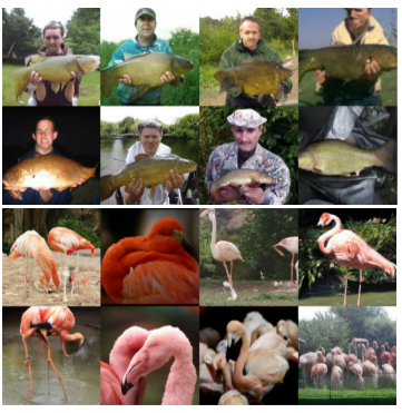
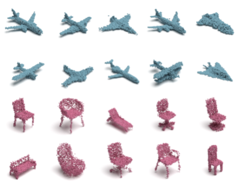
In the first half of 2021, a few papers popped up on arXiv claiming that a new method, motivated by non-equilibrium statistical physics (Sohl-Dickstein et al., 2015), achieved sample qualities better than contemporary state-of-the-art models. Here are some generated samples taken directly from these papers.

ImageNet 256 (Dhariwal & Nichol, 2021)	ShapeNet dataset (Luo & Hu, 2021)

I read about denoising diffusion probabilistic models (DDPM) while preparing to present to my colleagues at our weekly Rainbow ML reading group. I spent more time than I routinely would since some derivations were not easy to follow. Moreover, you can find a detailed explanation only in a handful of involved papers (Ho et al., 2020; Sohl-Dickstein et al., 2015). So I hope this post will provide a general understanding to a broader audience.

High-level overview

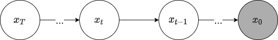
Given a data sample \(\boldsymbol{x_0}\), DDPM attempts to model the data distribution by introducing \(T\) latents \(\boldsymbol{x}_1, \boldsymbol{x}_2, ..., \boldsymbol{x}_T\), with a model parameterized by \(\theta\),

where \(d\boldsymbol{x}_{1:T}\) is just \(d\boldsymbol{x}_1 d\boldsymbol{x}_2 ... d\boldsymbol{x}_T\). Here, the factorization of the joint distribution is possible since the model is given by the following Markov chain,

To optimize our parametric model, we would like to compute the exact marginal likelihood and maximize it. Unfortunately, the exact likelihood (given by the above integral) is not tractable, and we are forced to resort to a variational approximation. During my first pass of a DDPM paper (Dhariwal & Nichol, 2021), I found this part particularly hard to follow and was forced to backtrack and read some earlier works. In this post, we will see how to start with the objective of minimizing a divergence between the approximate and true posterior, and pry out the evidence lower bound (ELBO). This is, of course, variational inference, and just in case you need a reminder (or are hearing about it for the first time), here is a brief outline of how it is typically carried out.

A primer on variational inference

The forward model is often quite simple, consisting of a single latent and a single observed variable. This results in a very simple graphical model,

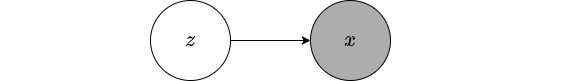
The posterior \(p(\boldsymbol{z} \vert \boldsymbol{x})\) is, in general, intractable and we resort to using an approximation \(q_\phi(\boldsymbol{z} \vert \boldsymbol{x})\), parameterized by \(\phi\). We optimize \(\phi\) by minimizing the KL-divergence between our approximate distribution and the true posterior \(D_\textrm{KL}(q_\phi(\boldsymbol{z} \vert \boldsymbol{x}) \, \| \, p(\boldsymbol{z} \vert \boldsymbol{x}))\). It turns out that this is equivalent to maximizing the evidence lower bound (ELBO) given by,

To better understand what is happening, an analogy I like using is that of trying to guess the mental state \(\boldsymbol{z}\) of a cat (or a dog if you prefer) based solely on its observed behavior \(\boldsymbol{x}\). None of us have any experience of being a cat and thus, have no priors about its mental states given its behavior \(p(\boldsymbol{z} \vert \boldsymbol{x})\). Instead, we anthropomorphize our furry friends and try to assign human-like mental states \(q(\boldsymbol{z} \vert \boldsymbol{x})\) because we know how to model these. However, it is important to note that these are approximations at best. The final step is assigning a mapping between certain mental states and certain observed behaviors based on real-world interactions, a process that is roughly equivalent to learning model parameters from data. We learn to infer that when a cat sits on our keyboards, it might be “craving attention” or that a dog wagging its tail is “most likely happy”.

I do not want to detail the derivation of obtaining the ELBO for the simple model described above since you can find several lecture notes and blog posts on it. Feel free to refer to them before reading on. In the rest of this post, I will elucidate how to do so for diffusion models.

Forward diffusion process

To better motivate the diffusion process, DDPM papers flip the “direction”. As a result, this is the picture you will see in most related work:

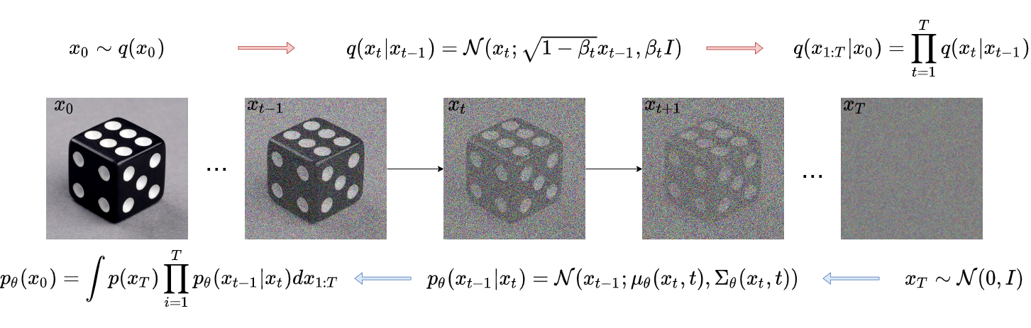
The forward process starts with an image taken from the training set and degrades it by iteratively adding small quantities of noise. The exact distribution of noise is known beforehand. After infinite iterations, all the information in the image is lost, and we are left with random noise. Formally, the forward diffusion process refers to extracting latents \(\boldsymbol{x}_1, \boldsymbol{x}_2, ..., \boldsymbol{x}_T\) from a given data sample \(\boldsymbol{x}_0 \sim q(\boldsymbol{x}_0)\). This is a well-defined process given by

Here \(\beta_t\) is provided by a predetermined variance schedule. After a large number of such diffusion steps, the final latent follows a standard Gaussian distribution \(\boldsymbol{x}_T \sim \mathcal{N}(0, \mathbf{I})\), from which we know how to efficiently sample. In practice, (Nichol & Dhariwal, 2021) show that between 1000 and 4000 steps are sufficient even for a complex distribution such as ImageNet.

Reverse diffusion process

The reverse process of generating a new sample boils down to inverting all diffusion steps each given by the posterior \(q(\boldsymbol{x}_{t-1} \vert \boldsymbol{x}_t, \boldsymbol{x}_0)\). Take a minute to realize that each inversion requires knowledge of the original data distribution. To understand why it helps to pay attention to a single diffusion step in isolation. While the forward process takes as input a slightly noisy image and adds a small amount of additional noise, the reverse inverts this operation. It should be obvious that estimating and removing the noise added in a diffusion step is a significantly more challenging task. To successfully reduce noise in an image, the model used should have a good prior of how noise-free images appear. Obviously, this is not available before training since \(q(\boldsymbol{x}_0)\) is precisely what we are interested in obtaining.

The choice of the forward diffusion operation, however, ensures that the posterior of each step is Gaussian, enabling us to easily approximate it. The Gaussian has only two parameters that need to be estimated and we do so with a model parameterized by \(\theta\),

This description is slightly different from the typical variational inference setup where an approximate model is used to obtain latents given the data. Here, the approximate model provides the data given the latents. The procedure remains the same—obtain a lower bound on the marginal log-likelihood of the data and update the parameters of a model to maximize it.

Evidence lower bound

Generally, latent variable models approximate the posterior of the latents, \(p(\boldsymbol{x}_{1:T}|\boldsymbol{x}_0)\) with a parameterized function. However, as we saw in the previous section, this approximation is predetermined when using diffusion methods. Instead, we learn the inversion of this process, \(p_\theta(\boldsymbol{x}_0|\boldsymbol{x}_{1:T})\) using the ELBO. Pay attention to the fact that the parameterization is now on the generative probability while the “approximate” posterior probability is well-defined. To derive the ELBO, we start with the objective of minimizing the KL-divergence between the approximate and true posteriors,

where we obtained the final step by extracting the marginal log-likelihood (since it does not depend on \(q\)), flipping the fraction inside the log function, and rearranging. The ELBO turns out to be a summation of several terms,

The formulation of diffusion models means that each intermediate probability \(p_\theta(\boldsymbol{x}_t)\), as well as \(q(\boldsymbol{x}_t)\). is a Gaussian. The final loss \(L = \Sigma_{t=0}^TL_t\) is thus a sum of many terms where all but one are KL-divergences between Gaussians. There are a few more caveats to optimizing this loss, but you will have to look at the papers for details (Ho et al., 2020; Nichol & Dhariwal, 2021).

Practical considerations

• Since each diffusion step adds Gaussian noise according to a predetermined schedule and Gaussians are closed under multiplication, we can directly sample an intermediate noisy image from \(q(\boldsymbol{x}_t \vert \boldsymbol{x}_0)\). Not having to iteratively perform every diffusion step vastly speeds up training.
• For generating new data after training, earlier papers recommended starting with a randomly drawn sample and going through the entire reverse diffusion operation iteratively. However, recent works (Song et al., 2020; Nichol & Dhariwal, 2021) demonstrate that this is not essential, and high-quality novel samples can be obtained with as few as 50 diffusion steps.
• The best results, with the highest likelihoods, are class-conditional samples. A few different approaches for conditioning (Dhariwal & Nichol, 2021; Luo & Hu, 2021) are possible.

References

1. Sohl-Dickstein, J., Weiss, E., Maheswaranathan, N., & Ganguli, S. (2015). Deep unsupervised learning using nonequilibrium thermodynamics. International Conference on Machine Learning, 2256–2265.
2. Dhariwal, P., & Nichol, A. (2021). Diffusion models beat gans on image synthesis. ArXiv Preprint ArXiv:2105.05233.
3. Luo, S., & Hu, W. (2021). Diffusion probabilistic models for 3d point cloud generation. Proceedings of the IEEE/CVF Conference on Computer Vision and Pattern Recognition, 2837–2845.
4. Ho, J., Jain, A., & Abbeel, P. (2020). Denoising diffusion probabilistic models. ArXiv Preprint ArXiv:2006.11239.
5. Nichol, A., & Dhariwal, P. (2021). Improved denoising diffusion probabilistic models. ArXiv Preprint ArXiv:2102.09672.
6. Song, J., Meng, C., & Ermon, S. (2020). Denoising diffusion implicit models. ArXiv Preprint ArXiv:2010.02502.